Efficient 4DGS Model Compression Using a Spatiotemporal KNN Algorithm

Ⅰ. Introduction

Recently, Implicit Neural Representations (INR)^[1], which represent 3D video through neural networks based on Neural Radiance Fields (NeRF)^[2], have gained attention as new technologies for 3D video representation and compression. INR models are learned via Multi-Layer Perceptrons (MLP) and can synthesize novel dynamic scenes at various time frames and viewpoints using learned neural networks. To improve both the rendering speed and quality of 3D representation models, hybrid methods^[3] that combine implicit and explicit representations, such as voxel grids, have also been explored. However, despite the acceleration of the rendering process through hybrid methods, there are still limitations in real-time processing of 3D videos.

3D Gaussian Splatting (3DGS)^[4] was originally developed as a technology optimized for real-time rendering of static 3D scenes. 3DGS results in faster rendering speeds compared to NeRF-based models by utilizing only explicit representation with 3D Gaussians. More recently, a dynamic model [5], [8] incorporating a temporal dimension into the 3DGS framework has emerged. In [5], a canonical space is utilized to extend the static capabilities of 3DGS, enabling the handling of dynamic scenes. Another new approach for representing 3D dynamic scenes is based on the Spacetime Gaussian (STG), which extends 3D Gaussians into the 4D spacetime domain^[8]. The STG model integrates 3D Gaussians and temporal elements to represent changes in dynamic scenes, such as object emergence and motion, and captures temporal variations using time-based parameters and temporal radial basis functions.

Meanwhile, the Moving Picture Experts Group (MPEG) has been evaluating implicit neural representations, hybrid representations, and explicit representations as new approaches for 2D/3D static and dynamic video representation and compression. To explore potential standardization, the Implicit Neural Visual Representation (INVR) Ad-hoc Group (AhG)^[6] is conducting Exploration Experiments (EEs)^[7]. EE2 focuses on investigating technologies to train and compress 6DoF (Degrees of Freedom) video using 3D INVR models. EE2.1 addresses NeRF-based implicit neural models and hybrid representations, while EE2.2 explores 3DGS techniques that explicitly represent static 3D scenes and dynamic 3DGS models, including a temporal dimension.

This paper presents a compaction method for the STG model^[8], which is a dynamic 3DGS model corresponding to INVR EE2.2. The STG model includes a preprocessing step that uses K-Nearest Neighbors (KNN) to group Gaussians along the same time axis and remove the top 25% of the closest pairs based on the distance between Gaussians before training. However, despite this preprocessing step, the resulting model still occupies approximately 29MB of memory, indicating that further compression techniques are required to make the STG model memory efficient.

In this paper, the Gaussians present at each timestamp undergo a preprocessing step that removes Gaussians based on spatial correlation, as in [8]. Additionally, the KNN algorithm is applied spatiotemporally to compact the model while representing Gaussians that have been created or disappeared during training. Following the Common Test Condition (CTC) of INVR EE 2.2, we train the STG model using the Mirror^[7] sequence from the MIV (MPEG Immersive Video) dataset, which consists of multi-view videos. The results obtained from the proposed compaction method are compared to those from models trained without preprocessing and with preprocessing. Additionally, when applying the proposed method to the STG model, we compare the compression results based on two criteria: scale and time distance. The proposed method demonstrates superior compression performance relative to rendering quality compared to existing techniques.

In Section 2, we introduce the 3DGS model, which uses explicit representation to model static 3D scenes, and the STG model, which extends the static characteristics of 3DGS by incorporating a temporal dimension. In Section 3, a compaction method for the STG model that utilizes spatiotemporal KNN is presented. Section 4 details the experimental results of the proposed method, and Section 5 concludes the paper.

Ⅱ. 3DGS and STG

1. 3DGS for static scene representation

3DGS^[4] is a representative explicit model that utilizes 3D Gaussians to represent 3D space. It converts multi-view images captured from various positions and angles into point clouds using Structure from Motion (SfM), with these points serving as the centroid of the 3D Gaussians.

Figure 1 illustrates the learning process of the 3DGS model. The point clouds are used to initialize the 3D Gaussians. The volume of each Gaussian can be represented by a covariance matrix, which can be decomposed into scale and rotation matrices to represent the transformed Gaussians during training. The color values are represented by Spherical Harmonics (SH) coefficients, with a higher degree of SH coefficients allowing for more detailed color representation. During the rendering process, the 3D Gaussians are projected onto a 2D plane. The 2D Gaussians are sorted in depth order for each pixel and accumulated to generate the rendered image. In addition, a densification process is applied to clone or split the Gaussians to fit the corresponding area. The parameters of each Gaussian, such as position, rotation, scale, color, and opacity are trained to minimize the difference between the rendered view and the provided multi-view images.

Fig. 1.

3DGS model training process[4]

2. STG for dynamic scene representation

3DGS is optimized for the real-time representation of static 3D scenes, leading to the development of several dynamic models that incorporate a temporal dimension into the structure of 3DGS. Figure 2 shows one of these dynamic models^[5]. In this model, 3D space is constructed using explicit representations of 3D Gaussians, with changes in position, rotation, and scale of each 3D Gaussian expressed through a deformation field. The deformation field is combined into a single vector processed by an MLP to capture temporal differences. A 3D canonical space is divided into a voxel grid and decomposed into six multi-resolution planes. The model connects adjacent Gaussians using a spatiotemporal structure encoder to predict their motion. However, since this structure is fundamentally based on forming a 3D canonical space and adding changes over time, it has limitations when objects exhibit significant changes.

Fig. 2.

Dynamic model based 3DGS model[5]

To address this issue, the STG model presents a new representation by including the temporal dimension directly within the 3D Gaussians, thereby modeling 4D Gaussians without relying on a 3D canonical space.

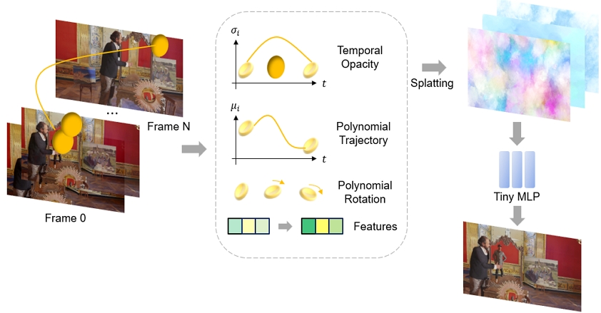
Figure 3 shows the entire learning process of the STG model. The STG model represents temporal opacity using 1D Gaussians, where opacity decreases as the difference between the prominent timestamp and the current timestamp increases. Polynomial functions model changes in position and rotation, allowing Gaussians to form trajectories over time. For color representation, instead of SH coefficients, the STG model uses basic RGB values along with features for viewing direction and time. These features are splatted to image space and categorized, with the final pixel intensity generated through a two-layer MLP. This approach results in a more compact model with fewer parameters than traditional SH coefficient encoding.

Fig. 3.

Learning process of Spacetime Gaussian (STG)

Table 1 compares the number of parameters for the 3DGS and STG models. The time component of the STG model includes the coefficients of polynomials that define position and rotation, as well as the prominently displayed timestamp and time scale. Therefore, the STG model can represent dynamic scenes with fewer parameters than the 3DGS model.

Table 1.

The number of parameters in the 3DGS and STG model configurations

Ⅲ. STG compaction using KNN algorithm

To represent a 4D dynamic scene, the STG model takes the form of a temporal component combined with 3D Gaussians. Also, the STG model applies a preprocessing step [8], in which the KNN algorithm is used to derive pairs composed of the spatially closest Gaussians for each timestamp. The distances between each pair are then measured and sorted in ascending order. The top 25% of these closest Gaussian pairs are removed as pairs, effectively reducing the total number of Gaussians. However, even after this existing preprocessing, the size of the trained model remains approximately 29MB, indicating that significant memory capacity is still required. Therefore, a more efficient method for removing Gaussians is needed. To address this issue, this paper proposes an efficient pruning method for STG model compaction by applying the KNN algorithm spatiotemporally.

1. Applying KNN algorithm spatiotemporally

In the existing method of the STG model, the KNN algorithm is applied independently for each timestamp, considering only spatial correlations while neglecting the temporal correlations between Gaussians. To account for the temporal relationships among Gaussians, we utilize the equations for the position and rotation of the STG model.

$\[ \begin{array}{c}{\mu }_i\left(t\right)\begin{array}{l}=\sum _{k=0}^{n_p}{b}_{i,k}{\left(t-{\mu }_i^{\tau }\right)}^k\hfill \\ =\begin{array}{l}{\mu }_i^s+b_{i,1}\left(t-{\mu }_i^{\tau }\right)+b_{i,2}{\left(t-{\mu }_i^{\tau }\right)}^2+\hfill \\ b_{i,3}{\left(t-{\mu }_i^{\tau }\right)}^3\hfill \end{array}\hfill \end{array}\hfill \end{array} \]$

(1)

$\[ q_i\left(t\right)\begin{array}{l}=\sum _{k=0}^{n_q}{c}_{i,k}{\left(t-{\mu }_i^{\tau }\right)}^k\hfill \\ =\begin{array}{l}{q}_i^s+c_{i,1}\left(t-{\mu }_i^{\tau }\right)+c_{i,2}{\left(t-{\mu }_i^{\tau }\right)}^2+\hfill \\ c_{i,3}{\left(t-{\mu }_i^{\tau }\right)}^3\hfill \end{array}\hfill \end{array} \]$

(2)

In equations (1) and (2), $$ {\mu }_i^{\tau }$$ represents the timestamps when the Gaussians are most prominently displayed. The initial value of $$ {\mu }_i^{\tau }$$ is determined based on the temporal axis of the frame to which the Gaussian belongs. As training progresses, the opacity is optimized, and accordingly, the value of $$ {\mu }_i^{\tau }$$ also changes. $$ {\mu }_i^s$$ and $$ q_i^s$$ represent the positions and rotations of the Gaussians at timestamp $$ {\mu }_i^{\tau }$$. n_p and n_q are hyper parameters that determine the degree of the polynomial. Higher values for these parameters increase the capacity to represent temporal changes but also increase the model size. b_i,k and c_i,k are the coefficients modeling the changes over time, respectively. As the current timestamp diverges from $$ {\mu }_i^{\tau }$$, the changes in position and rotation increase.

We use the KNN algorithm to select Gaussians at timestamp $$ {\mu }_i^{\tau }$$ that share the same nearest neighbors in positions and rotations. The same approach is applied at the current time t, achieving spatial correlations for each timestamp. To establish temporal correlations, we select pairs of Gaussians that share the same nearest neighbors across both timestamps. This indicates that the nearest Gaussians are consistent when each is most visible and changes over time, suggesting that the matched pairs have similar time trajectories. Additionally, each pair follows the index of the reference Gaussian input to KNN. In other words, the indices of each pair match the order of the reference Gaussians input to KNN.

Figure 4 shows the process of applying the spatiotemporal KNN algorithm to the STG model. As shown in Figure 4, Gaussians A, B, and C change in position and rotation over time. The timestamps when each Gaussian is most prominently displayed are denoted as $$ {\mu }_A^{\tau }$$, $$ {\mu }_B^{\tau }$$, and $$ {\mu }_C^{\tau }$$ respectively. Taking Gaussian A as the reference, when the timestamp is $$ {\mu }_A^{\tau }$$, the closest neighbor in terms of position is Gaussian B, which also exhibits the most similar rotation. When considering the timestamp t, the changes in position and rotation of Gaussian A are most similar to those of Gaussian B. Therefore, efficient pruning can be achieved by replacing two Gaussians with similar temporal trajectories with one.

Fig. 4.

Process of spatiotemporal KNN algorithm

2. Adaptive pruning based on rendering loss

In the preprocessing of the STG model, the distances between the matched Gaussian pairs, determined by the KNN algorithm, are calculated and sorted in ascending order. The top 25% of these Gaussian pairs are then removed based on their proximity. This method assumes that spatially close Gaussians share similar characteristics. Although the KNN algorithm already pairs spatially adjacent Gaussians, sorting the Gaussian pairs based on proximity allows for further selection of the closest pairs to reduce redundancy. However, applying this method during training results in the removal of a significant number of Gaussians, which can fall short of the minimum number required to accurately represent a 3D scene, leading to noticeable degradation in rendering quality. Therefore, in the design of the proposed method, a more suitable criterion for removing Gaussians from the matched pairs is required.

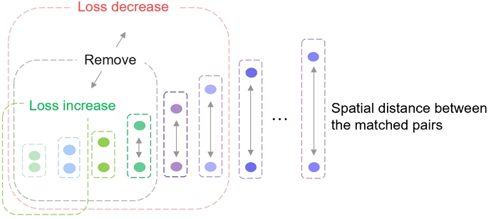
Figure 5 illustrates the proposed method, where the removal rate for the matched Gaussian pairs is adaptively adjusted based on the rendering quality loss. After the distances between the matched Gaussian pairs are sorted in ascending order, if the rendering loss increases, the removal rate decreases, and if the rendering loss decreases, the removal rate increases. In this approach, maximum and minimum thresholds are set for the removal rate to prevent excessive removal of Gaussians while reducing redundancy, ensuring that enough Gaussians remain to maintain scene rendering quality. In this way, the Gaussian pairs to be removed are selected based on the closest distances according to the determined rate.

Fig. 5.

Adaptive pruning based on the rendering loss

Ⅳ. Experimental results

In the experiments, the STG model^[8] is trained using the Mirror sequence^[7], which consists of 15 multi-view videos, following the INVR CTC. Each video has a duration of 3 seconds at 32 frames per second, and the training is conducted over 1 second using all views except for two test views (v06 and v08). During training, the proposed method is applied, and the test views are rendered using the trained model to evaluate compression efficiency based on compression ratio and rendering quality. Performance is assessed by comparing Bit-Per-Second (BPS), which represents the number of bits transmitted per second, with the Peak Signal-to-Noise Ratio (PSNR) of the rendered test views’ quality.

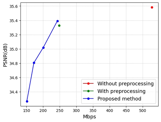
Table 2 presents a comparison of the BPS-PSNR performance between the trained STG model with and without preprocessing, as well as the STG model trained with the proposed pruning method. The pruning method is applied every 100 training iterations, with training ranges defined as {Case 1, Case 2, Case 3, Case 4}, where the range progressively increases from Case 1 to Case 4. In Case 1, pruning is applied from 6k to 12k iterations; in Case 2, from 6k to 16k; and in subsequent cases, the pruning range increases by 4k iterations, up to Case 4. Figure 6 illustrates the Rate-Distortion (RD) curves corresponding to the results in Table 2.

Table 2.

BPS-PSNR performance comparison of the proposed method and w/wo preprocessing for the trained STG model

Fig. 6.

BPS-PSNR performance comparison

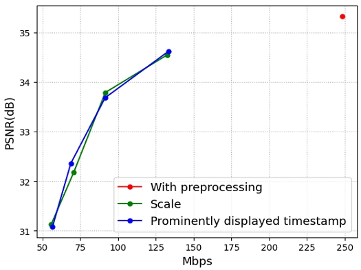
Table 3 compares the BPS-PSNR performance when applying scale and prominently displayed timestamp as criteria for removing Gaussians in the preprocessed model. The proposed method and comparison methods all render the same test views from the same multi-view video sequences. Figure 7 presents the RD curves for the results in Table 3. From the results, it can be observed that the proposed method achieves superior BPS-PSNR performance compared to existing approaches.

Table 3.

Experimental results on the comparison of BPS-PSNR performances

Fig. 7.

BPS-PSNR performance comparison

The experimental results demonstrated that preprocessing in the existing STG model^[8] effectively pruned Gaussians at each timestamp, leveraging spatial correlations. Moreover, applying the proposed method during training showed superior BPS-PSNR performance. In the quantitative results, compared to the trained STG model, the proposed method achieves a 54% reduction in model size with only a 0.2 dB decrease in PSNR. Additionally, when compared to the trained STG model with preprocessing, the proposed method reduces the model size by 2.26% while yielding a 0.07 dB improvement in PSNR.

However, there was no significant difference in BPS-PSNR performance between the models that selected Gaussians based on scale and the prominently displayed timestamp. While the timestamp is an important factor representing the temporal continuity of Gaussians, the results confirmed that the key information of the scene is primarily determined by spatial characteristics. In summary, although a lower prominent timestamp may better represent the initial scene, it does not always result in a significant improvement in PSNR rendering quality.

Ⅴ. Conclusion

In this paper, we propose an efficient compaction method of the STG model, an explicit representation model, aimed at enhancing the compression of 6DoF immersive video. Initially, spatial compaction is applied to the STG through preprocessing. Then, during dynamic multi-view training, the proposed method performs spatiotemporal pruning. This approach enables the efficient representation of dynamic 3D scenes while achieving efficient compaction. The proposed method outperforms the existing model in terms of BPS-PSNR performance. Additionally, this method can be applied to various dynamic 3DGS models utilizing explicit representation, offering significant potential for compressing 6DoF immersive video through enhanced representation and compaction in dynamic 3DGS models.

Acknowledgments

This work was supported by the IITP grant (No. 2018-0-00207, Immersive Media Research Laboratory) and the NRF grant (No. RS-2024-00356924), both funded by the Korea government (MSIT).

References

• V. Sitzmann, J. N. P. Martel, A. W. Bergman, D. B. Lindell, and G. Wetzstein, “Implicit neural representations with periodic activation functions,” Advances in Neural Information Processing Systems, vol. 13, pp.7462–7473, 2020. [https://doi.org/10.48550/arXiv.2006.09661]
• B. Mildenhal, P. P. Srinivasan, M. Tancik, J. T. Barron, R. Ramamoorthi, and R. Ng, “Nerf: Representing Scenes as Neural Radiance Fields for View Synthesis,” Proceedings of the European Conference on Computer Vision, pp. 405-421, Aug. 2020. [https://doi.org/10.1007/978-3-030-58452-8_24]
• S. Fridovich-Keil, A. Yu, M. Tancik, Q. Chen, B. Recht, and A. Kanazawa, “Plenoxels: Radiance Fields without Neural Networks,” Proceeding of the IEEE Conference on Computer Vision and Pattern Recognition, pp. 5501–5510, 2022. [https://doi.org/10.1109/CVPR52688.2022.00542]
• B. Kerbl, G. Kopanas, T. Leimkühler, and G. Drettakis, “3D Gaussian Splatting for Real-Time Radiance Field Rendering,” ACM Transactions on Graphics, vol.42, No.4, pp.1–14, 2023. [https://doi.org/10.1145/3592433]
• Guanjun Wu, Taoran Yi, Jiemin Fang, Lingxi Xie, Xiaopeng Zhang, Wei Wei, Wenyu Liu, Qi Tian and Xinggang Wang, “4D Gaussian Splatting for Real-Time Dynamic Scene Rendering,” arXiv preprint arXiv:2310.08528, 2023. [https://doi.org/10.48550/arXiv.2310.08528]
• G. Lafruit, Y. Liao, and G. Bang, AhG on Implicit Neural Video Representations (INVR), ISO/IEC JTC1/SC 29/WG04, M60641, Oct. 2022.
• Y. Liao, and G. Bang, BoG report on Implicit Neural Visual Representation (INVR), ISO/IEC JTC 1/SC 29/WG04, M68163, Apr. 2024.
• Z. Li, Z. Chen, Z. Li, and Y. Xu, “Spacetime gaussian feature splatting for real-time dynamic view synthesis,” Proceeding of the IEEE Conference on Computer Vision and Pattern Recognition, pp. 8508–8520. 2024. [https://doi.org/10.48550/arXiv.2312.16812]
• J. C. Lee, et al. “Compact 3d gaussian splatting for static and dynamic radiance fields.” arXiv preprint arXiv:2408.03822, 2024. [https://doi.org/10.48550/arXiv.2408.03822]